
दोस्तों, क्या कभी ऐसा हुआ है कि आपने Excel में salary का data enter किया — लेकिन numbers plain दिख रहे हों, कोई ₹ sign नहीं, कोई comma नहीं? या date को DD/MM/YYYY में दिखाना था लेकिन Excel ने कुछ और format में दिखा दिया? या फिर किसी important cell को highlight करना था लेकिन वो बाकी सब cells जैसी plain दिख रही थी? यह सब problems एक ही जगह से solve होती हैं — Format Cells। आज हम सीखेंगे Excel mein Format Cells kaise use kare — पूरी detail में, हर tab को, हर option को।
Format Cells की सबसे खास बात यह है कि इससे cell की original value नहीं बदलती — सिर्फ वो कैसे दिखती है, यह बदलता है। यानी 0.5 enter करे और Percentage format लगाये तो वो — दिखेगा 50%, लेकिन असल value 0.5 ही रहेगी।

Format Cells क्या है? — फॉर्मेट सेल की पूरी जानकारी
Format Cells Excel का एक dialog box है जिसकी सहायता से हम किसी भी cell में enter की गई value के रूप-रंग (appearance) को बदल सकते हैं — बिना उसके value को बदले।
Format Cells के अंदर हम 6 अलग-अलग प्रकार के काम कर सकते हैं:
- Number Formatting — Numbers को Currency, Percentage, Date, Time आदि में दिखाना
- Alignment — Text को Left, Right, Center, या Wrap करना
- Font — Font का style, size, color बदलना
- Border — Cell के चारों तरफ border लगाना
- Fill — Cell का background color या pattern बदलना
- Protection — Cell को lock या hide करना
सबसे जरूरी बात: Format Cells से cell की original value कभी नहीं बदलती। उदाहरण — 0.5 को Currency format में ₹0.50 दिखेगा, Percentage में 50% दिखेगा — लेकिन formula bar में हमेशा 0.5 ही दिखेगा। यही Excel की formatting की असली power है।
Format Cells Dialog Box कैसे खोलें? 💡
Format Cells dialog box खोलने के कई तरीके हैं:
| तरीका | Steps | सबसे Fast? |
|---|---|---|
| Keyboard Shortcut | Cell select करें → Ctrl+1 press करें | ✅ सबसे Fast! |
| Right-Click Menu | Cell पर Right-Click → “Format Cells” select करें | Easy |
| Home Tab से | Home Tab → Number Group → छोटा arrow (Dialog Box Launcher) click करें | — |
| Ribbon से | Home Tab → Cells Group → Format → Format Cells | — |

| Category | क्या करती है | Example |
|---|---|---|
| General | Default format — कोई specific formatting नहीं | 1234.5 |
| Number | Decimal places और comma separator set करना | 1,234.50 |
| Currency | Currency symbol के साथ amount | ₹1,234.50 |
| Accounting | Currency symbol aligned, negatives में brackets | ₹ 1,234.50 |
| Date | Date को अलग-अलग formats में दिखाना | 01/01/2025 या January 1, 2025 |
| Time | Time format — 12-hr या 24-hr | 2:30 PM या 14:30 |
| Percentage | Number को % में convert करके दिखाना | 0.5 → 50% |
| Fraction | Decimal को fraction में दिखाना | 0.5 → 1/2 |
| Scientific | Scientific notation में | 1234500 → 1.23E+06 |
| Text | Number को text की तरह treat करना | 001 (leading zeros) |
| Special | Phone number, Zip code formats | +91-9876543210 |
| Custom | अपना खुद का format बनाना | कोई भी custom pattern |

Tab 2 — Alignment Tab (Text Alignment)
Alignment Tab से cell के अंदर text की position और direction control की जाती है। यह tab बहुत काम का है जब आप data को visually clean और readable बनाना चाहते हों।
Alignment Tab में मुख्य options:
Horizontal Alignment
- General — Text left, Numbers right (default)
- Left — सब कुछ left side में
- Center — center में align
- Right — right side में
- Fill — cell को पूरा fill करे character से
- Justify — दोनों sides में evenly spread
- Center Across Selection — Merge किए बिना center में दिखाना
Vertical Alignment
- Top — cell के ऊपर
- Middle — cell के बीच में
- Bottom — cell के नीचे (default)
Text Control — बहुत Important!
- Wrap Text — लंबा text एक cell में wrap होगा (नई line में जाएगा)
- Shrink to Fit — text को cell में fit होने के लिए automatically छोटा करता है
- Merge Cells — multiple cells को एक में merge करता है
Orientation (Text Direction)
Text को 90 degree घुमाना हो, vertical करना हो — Orientation option से होता है। Headers में यह बहुत useful है।
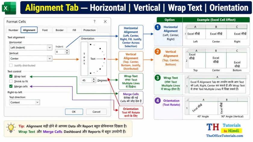
Wrap Text vs Merge Cells: Merge Cells से cells एक हो जाती हैं — लेकिन बाद में sorting और formulas में problem आती है। इसलिए जहाँ possible हो, Wrap Text use करें — cells अलग रहती हैं लेकिन text properly दिखता है।
Tab 3 — Font Tab (Font Styling)
Font Tab से cell के text का style, size, color और effects बदले जाते हैं। Home Tab से भी यह सब होता है — लेकिन Format Cells के Font Tab में ज्यादा options मिलते हैं।
Font Tab के मुख्य options:
- Font — Arial, Calibri, Times New Roman आदि — अपनी पसंद का font
- Font Style — Regular, Italic, Bold, Bold Italic
- Size — Font का size (points में)
- Underline — Single, Double, Single Accounting, Double Accounting
- Color — Text का color
- Effects:
- Strikethrough — text के बीच से line (जैसे
यह) - Superscript — ऊपर छोटा text (जैसे m²)
- Subscript — नीचे छोटा text (जैसे H₂O)
- Strikethrough — text के बीच से line (जैसे
Accounting Underline: Normal underline और Accounting Underline में फर्क है। Accounting Underline cell की पूरी width में जाती है — financial statements में use होती है।

Tab 4 — Border Tab (Cell Border)
Border Tab से cells के चारों तरफ lines (borders) लगाई जाती हैं। Plain Excel sheet professional लगे — इसके लिए proper border formatting जरूरी है।
Border Tab के Sections:
Presets (Ready-made options):
- None — सभी borders हटा दो
- Outline — सिर्फ बाहरी border
- Inside — सिर्फ अंदरूनी lines (multiple cells select करने पर)
Border (Manual control):
- Top, Bottom, Left, Right — अलग-अलग sides पर border
- Diagonal borders — cells में cross lines
Line Style और Color:
- पतली, मोटी, dotted, dashed, double line — कोई भी style choose करें
- Border का color भी change कर सकते हैं
Step to Apply:
- Cells select करें जिनमें border लगानी हो।
- Ctrl+1 press करें → Border Tab पर click करें।
- Line Style choose करें — पहले style choose करें, फिर border apply करें।
- Color choose करें (optional)।
- Presets से Outline या Inside click करें — या manually individual sides click करें।
- OK click करें।

जरूरी बात: Border Tab में पहले Line Style और Color choose करें — फिर border apply करें। अगर पहले border apply किया और फिर style बदला, तो बदलाव नहीं होगा।
Tab 5 — Fill Tab (Background Color)
Fill Tab से cell का background color, gradient और pattern set किया जाता है। Important data को highlight करना हो, headers को colorful बनाना हो — Fill Tab यहीं से होता है।
Fill Tab के Options:
- Background Color — Color palette से कोई भी color choose करें। “More Colors” से custom color (HEX code से) भी set कर सकते हैं।
- Fill Effects — Gradient fill — दो colors के बीच smooth transition। Professional-looking headers बनाने के लिए perfect।
- Pattern Style — Solid color की जगह dots, stripes जैसे patterns।
- Pattern Color — Pattern का color।
- No Color — Background color हटाना।
Step to Apply:
- Cell या range select करें।
- Ctrl+1 → Fill Tab।
- Background Color में से color choose करें।
- Gradient चाहिए तो Fill Effects पर click करें।
- OK click करें।

Tab 6 — Protection Tab (Cell Lock/Hide)
Protection Tab से cells को lock या hide किया जाता है — लेकिन यह तभी काम करता है जब sheet protect हो।
Protection Tab के Options:
- Locked — Default: सभी cells locked होती हैं। Sheet protect होने पर locked cells edit नहीं होंगी।
- Hidden — Formula bar में formula नहीं दिखेगा — formula hide हो जाएगा। Sheet protect होने पर।
कैसे Use करें:
- जो cells edit हो सकें — उन्हें select करें → Ctrl+1 → Protection → Locked uncheck करें।
- जो cells protect करनी हैं — उन्हें locked रहने दें।
- फिर Review Tab → Protect Sheet से sheet protect करें।
- अब locked cells edit नहीं होंगी, unlocked cells होंगी।
Important: Protection Tab का Locked/Hidden option तब तक काम नहीं करता जब तक Sheet Protect न हो। Sheet protect करने के बाद ही यह effective होता है।

Number Tab के Practical Examples — Commonly Used
अब देखते हैं कि Number Tab के popular formats practically कैसे apply करते हैं।
Example 1: 0.5 को ₹ (Currency) में बदलना
Step to Apply:
- Cell में 0.5 enter करें।
- Cell select करें → Ctrl+1 press करें।
- Number Tab already selected होगा।
- Category list में “Currency” click करें।
- Right side में Symbol dropdown से ₹ (Indian Rupee) choose करें।
- Decimal Places में 2 रखें।
- OK click करें।
Result: 0.5 → ₹0.50 दिखेगा। Formula bar में अभी भी 0.5 ही रहेगा।

Example 2: 0.5 को 50% (Percentage) में बदलना
Step to Apply:
- Cell में 0.5 enter करें।
- Ctrl+1 press करें।
- Category list में “Percentage” click करें।
- Decimal Places — 0 या 1 अपनी जरूरत के हिसाब से।
- OK click करें।
Result: 0.5 → 50% दिखेगा।
ध्यान दें: Excel में Percentage format इस तरह काम करता है — cell में जो value है उसे 100 से गुणा करके % sign लगाता है। इसलिए 0.5 → 50%, 1 → 100%, 0.25 → 25%। अगर आप 50 enter करके % format करोगे तो 5000% दिखेगा — सावधान रहें!

Example 3: Number को Date Format में दिखाना
Excel में dates internally numbers होती हैं। 1 = 01/01/1900। आप किसी number को date format दे सकते हैं।
Step to Apply:
- Cell में कोई number enter करें — जैसे 45292।
- Ctrl+1 → Number Tab → Category list में “Date” click करें।
- Right side में Type list से अपना preferred date format choose करें — जैसे DD/MM/YYYY।
- OK click करें।
Result: 45292 → 01/01/2024 दिखेगा।
Example 4: Custom Format — अपना खुद का Format बनाना
Custom format से आप कोई भी unique format create कर सकते हैं। जैसे numbers में “Units” suffix लगाना।
Category list में “Custom” select करें → Type field में format code लिखें:
| Custom Format Code | Value | Result |
|---|---|---|
#,##0 | 1234567 | 1,234,567 |
#,##0.00 | 1234.5 | 1,234.50 |
₹#,##0.00 | 1234.5 | ₹1,234.50 |
0.00"kg" | 45.5 | 45.50kg |
"Units: "#,##0 | 500 | Units: 500 |
DD/MM/YYYY | Date | 01/06/2025 |
DD-MMM-YYYY | Date | 01-Jun-2025 |

Format Cells के Shortcuts — Quick Reference
Format Cells को faster use करने के लिए ये shortcuts याद कर लें:
| Shortcut | क्या करता है |
|---|---|
| Ctrl+1 | Format Cells dialog box खोलना |
| Ctrl+B | Bold |
| Ctrl+I | Italic |
| Ctrl+U | Underline |
| Ctrl+Shift+$ | Currency format (default) |
| Ctrl+Shift+% | Percentage format |
| Ctrl+Shift+# | Date format (DD-MMM-YY) |
| Ctrl+Shift+@ | Time format |
| Ctrl+Shift+! | Number format (comma separator, 2 decimals) |
| Ctrl+Shift+~ | General format (formatting हटाना) |
| Alt+H+H | Fill Color (background) |
| Alt+H+FC | Font Color |
Time-Saving Tip: अगर एक cell पर formatting apply की है और दूसरी cell पर same formatting चाहिए — तो Format Painter (Ctrl+C → Alt+H+V+T) या simply Paint Bucket (F4) use करें।

Excel की और भी formatting features और functions सीखने के लिए देखें: Excel Formula और Function — Complete Guide और Excel Shortcut Keys — पूरी List
Format Cells की official Microsoft documentation यहाँ देखें: Microsoft Support — Format Cells Dialog Box
निष्कर्ष
तो दोस्तों, आज हमने पूरी detail में सीखा कि Excel mein Format Cells kaise use kare — Number, Alignment, Font, Border, Fill और Protection — सभी 6 tabs को उदाहरण के साथ। Format Cells Excel का एक ऐसा powerhouse feature है जिसे जानने के बाद आपकी spreadsheets कभी plain नहीं लगेंगी।
याद रखें — Ctrl+1 shortcut से Format Cells तुरंत खुलता है। Currency के लिए, Percentage के लिए, Date format के लिए — सब कुछ एक ही dialog box में है।
नीचे comment जरूर करें — Format Cells में कौन सा feature आपको सबसे ज्यादा काम आता है? कोई confusion हो तो भी पूछें। और TheOfficeTutorials.com को bookmark करना न भूलें — Excel के basics से advanced tips तक सब कुछ यहाँ मिलता है।
FAQ — अक्सर पूछे जाने वाले सवाल
Format Cells kaise khole Excel mein?
Format Cells खोलने के तीन तरीके हैं। सबसे fast — cell select करें और Ctrl+1 press करें। दूसरा — cell पर right-click करें और “Format Cells” select करें। तीसरा — Home Tab में Number Group के छोटे arrow पर click करें।
Format Cells se kya hota hai?
Format Cells से cell की value का appearance बदलता है — original value नहीं बदलती। इससे Number formatting (Currency, Percentage, Date), Text Alignment, Font styling, Border, Background color, और Cell Protection — सब कुछ एक dialog box में किया जा सकता है।
Excel mein number ko currency mein kaise badle?
Cell select करें → Ctrl+1 → Number Tab → Currency → Symbol dropdown से ₹ (Indian Rupee) choose करें → Decimal Places set करें → OK। या shortcut से: Ctrl+Shift+$ press करें — default currency format apply हो जाएगा।
Excel mein date format kaise change kare?
Date cell select करें → Ctrl+1 → Number Tab → Date → Type list में से desired format choose करें जैसे DD/MM/YYYY, DD-MMM-YY आदि → OK। Custom format के लिए Custom category में DD/MM/YYYY या DD-MMM-YYYY type करें।
Percentage format lagane ke baad galat result aa raha hai — kyun?
Excel में Percentage format cell value को 100 से multiply करके % sign लगाता है। इसलिए अगर आपने 50 enter किया और Percentage format लगाया तो 5000% दिखेगा। 50% के लिए cell में 0.5 enter करें, फिर Percentage format लगाएं।
Excel mein cell ka background color kaise change kare?
Cell select करें → Ctrl+1 → Fill Tab → Background Color में से color choose करें → OK। Quick shortcut: Home Tab में Fill Color button (paint bucket icon) से directly color select करें। Gradient के लिए Fill Tab → Fill Effects।
Format Cells ka Protection Tab kab kaam karta hai?
Protection Tab का Locked और Hidden option तभी काम करता है जब sheet protect हो। पहले cells को locked/unlocked set करें, फिर Review Tab → Protect Sheet से sheet protect करें। बिना sheet protect के Protection Tab settings का कोई effect नहीं होता।
Format Cells aur Home Tab formatting mein kya fark hai?
Home Tab पर commonly used formatting options quick access के लिए होते हैं — जैसे Bold, Italic, Font Color, Fill Color, Basic Number formats। Format Cells dialog box (Ctrl+1) में सभी formatting options ज्यादा detail में मिलते हैं — Custom formats, Accounting Underline, Gradient Fill, Diagonal Borders जैसी advanced settings।