
दोस्तों, Excel सीखने की शुरुआत में एक चीज़ है जो हर किसी को confuse करता है — और वो है Cell Reference। Formula लिखते वक्त हमको A1, $A$1, $A1, A$1 का उपयोग करना होता है — और यह सब देखकर मन घबराहट होती है। लेकिन सच यह है कि जैसे ही आप समझ जाते हैं कि Excel mein Cell Reference kya hai और यह कितने प्रकार का होता है — formulas लिखना बहुत आसान हो जाता है। आज इस tutorial में हम Cell Reference को एकदम शुरू से, उदाहरणों के साथ, step-by-step समझेंगे। 🎯
यह concept Excel के हर beginner के लिए जरूरी है — चाहे आप student हों, job seeker हों, या office में काम करते हों। एक बार यह समझ आ गया तो SUM, VLOOKUP, IF — कोई भी formula लिखना आसान लगने लगेगा।

Table of Contents
सेल एड्रेस क्या है? — What is Cell Address in Excel
Cell Reference के बारे में समझने के लिए सबसे पहले हमें यह समझना होगा कि Cell Address क्या है। तो आइए पहले यही समझते हैं।
Excel की Spreadsheet/Worksheet में Rows और Columns होते हैं। जहाँ एक Row और एक Column मिलते हैं — उस point को Cell कहते हैं। और उस Cell का एक unique नाम होता है जो उस worksheet में अद्वितीय (Unique) होता है — उसी को Cell Address कहते हैं।
Cell Address हमेशा Column Letter + Row Number के format में लिखा जाता है। Column का नाम और Row का नंबर एक साथ लिखने से Cell का Address बनता है। जैसे:
- C3 — इसमें C Column का नाम है और 3 Row का नंबर। यानी Column C और Row 3 का intersection — Cell Address: C3
- A1 — Column A, Row 1 का intersection।
- B5 — Column B, Row 5 का intersection।

Cell Range का Address क्या होता है?
जब आप एक से ज्यादा cells एक साथ select करते हैं तो उसे Cell Range कहते हैं। Range का address इस format में लिखा जाता है:
पहला Cell : आखिरी Cell — बीच में Colon (:) होता है।
कुछ उदाहरण देखें:
- C4:C8 — Column C में Row 4 से Row 8 तक — यानी C4, C5, C6, C7, C8 सब।
- B2:E5 — B2 पहला सेल और E5 आखिरी सेल — इस rectangular area में सभी cells आती हैं।
- A1:A10 — Column A में पहली 10 rows — SUM formula में अक्सर यही use होता है।

अब जब आप दो या दो से अधिक अलग-अलग rows और columns का selection करते हैं — तो पहला selected cell का address और आखिरी selected cell का address मिलकर range का address बनाते हैं। जैसे B2 से E5 तक select करने पर B2 पहला cell और E5 अंतिम cell माना जाएगा — Range Address: B2:E5
इसके बारे में विस्तार से पढ़ें: Cell Range (सेल रेंज) क्या है — पूरी जानकारी
Cell Reference क्या है? — Excel mein Cell Reference kya hai 🎯
जब कभी भी हम Excel में किसी Formula या Function का प्रयोग करते हैं — तो उस formula या function में Cell Reference (सेल सन्दर्भ) की जरूरत होती है। इसकी जगह पर हम Cell Address का उपयोग करते हैं — और यही Cell Address उस formula या function का Cell Reference बन जाता है।
सरल शब्दों में: Formula में किसी Cell का Address देना = Cell Reference।
उदाहरण: मेरे पास कुछ cells में कुछ numbers हैं जिनका योग निकालना है। अब हम SUM function का प्रयोग करेंगे और function के Cell Reference में उस cell range का address देंगे जहाँ numbers मौजूद हैं।
जैसे: A1 में 10 और B1 में 20 है। C1 में formula लिखें =SUM(A1,B1) — तो यहाँ A1 और B1 Cell References हैं। Result आएगा: 30।

Cell Reference का सबसे बड़ा फायदा यह है कि अगर A1 की value 10 से बदलकर 50 हो जाए — तो C1 का result automatically 30 से बदलकर 70 हो जाएगा। यही Excel की असली ताकत है — Dynamic Calculation।
Cell Reference क्यों जरूरी है? 💡
यह सवाल कई लोगों के मन में आता है — “Formula में directly number क्यों नहीं लिखते?” जैसे =10+20 लिखें तो भी तो 30 आएगा।
लेकिन सोचिए — अगर data बदल जाए तो क्या होगा?
- अगर आपने
=10+20लिखा है और data बदल गया — तो आपको formula manually edit करना होगा। - अगर आपने
=A1+B1लिखा है — तो A1 या B1 में जो भी value बदलो, result automatically update होगा।
Cell Reference के 4 बड़े फायदे:
| फायदा | कैसे काम करता है |
|---|---|
| Dynamic Update | Data बदलो — result automatically बदलता है |
| Formula Copy करना आसान | एक formula लिखो — पूरे column में copy करो |
| Errors कम होती हैं | Manual entry की जगह cell reference — typo की गुंजाइश नहीं |
| Large Data आसानी से handle होता है | 1000 rows का SUM = =SUM(A1:A1000) — एक formula |
सेल सन्दर्भ के प्रकार — Types of Cell Reference in Excel
Excel में Cell Reference को हम तीन भागों में बाँट सकते हैं:
- Relative Cell Reference — सापेक्ष सेल सन्दर्भ
- Absolute Cell Reference — निरपेक्ष सेल सन्दर्भ
- Mixed Cell Reference — मिश्रित सेल सन्दर्भ
| प्रकार | Example | क्या होता है | कब Use करें |
|---|---|---|---|
| Relative | A1 | Copy करने पर address बदल जाता है | जब formula को rows/columns में copy करना हो |
| Absolute | $A$1 | Copy करने पर address नहीं बदलता | जब एक fixed cell को हमेशा refer करना हो |
| Mixed | $A1 या A$1 | Column या Row में से एक lock, एक free | जब सिर्फ row या सिर्फ column lock करना हो |
आइए अब तीनों को detail में उदाहरण के साथ समझते हैं।
1. Relative Cell Reference — सापेक्ष सेल सन्दर्भ
Relative Cell Reference में वैसे Cell Address को लिया जाता है जो पहले से lock न किया हुआ हो। इसमें जब हम किसी cell में कोई formula के साथ दो या दो से अधिक Cell References दिए हों और जब आप वही formula किसी दूसरी cell में copy-paste करें — तो reference पुराने reference के अनुसार (Relatively) बदल जाता है।
यह Excel का default behavior है। जब आप simply A1 लिखते हैं बिना किसी $ के — वो Relative Reference होता है।
💡 सरल भाषा में: Relative Reference यह याद रखता है कि formula cell और referenced cell के बीच कितनी “दूरी” है — और copy होने पर वही दूरी maintain करता है।
Relative Cell Reference का उदाहरण
A1 और B1 में data है, C1 में =SUM(A1,B1) है। अब C1 को copy करके C2 में paste करते हैं।
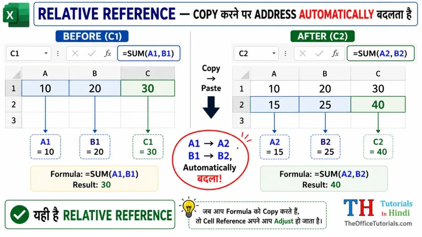
- C1 में formula था:
=SUM(A1,B1) - C1 को C2 में copy किया।
- C2 में Cell Reference बदल गया — अब C2 में
=SUM(A2,B2)हो गया। ✅
C1 से C2 में जाने पर एक row नीचे गए — तो A1 भी A2 हो गया और B1 भी B2 हो गया। यही Relative Reference की working है।
🎯 कब Use करें: जब आप एक ही formula को पूरे column या row में copy करना चाहते हों — जैसे Marksheet में हर student के marks का total निकालना, या Sales report में हर product की total sales calculate करना। Relative Reference सबसे ज्यादा use होने वाला reference है।
Relative Reference — एक Practical Example
मान लीजिए आपके पास 5 students की Marksheet है। हर student के Maths और Science के marks हैं — और आपको Total निकालना है:
| Student | Maths (Col B) | Science (Col C) | Total (Col D) |
|---|---|---|---|
| Rahul | 85 | 90 | =SUM(B2,C2) → 175 |
| Priya | 78 | 82 | =SUM(B3,C3) → 160 (auto) |
| Amit | 92 | 88 | =SUM(B4,C4) → 180 (auto) |
| Neha | 70 | 75 | =SUM(B5,C5) → 145 (auto) |
| Ravi | 88 | 91 | =SUM(B6,C6) → 179 (auto) |
D2 में formula लिखा — D3 से D6 तक copy किया। Relative Reference की वजह से हर row में formula automatically adjust हो गया। सिर्फ एक formula — 5 rows का काम। यही है Relative Reference की power!
2. Absolute Cell Reference — निरपेक्ष सेल सन्दर्भ
जब हम formula में उपयोग होने वाले Cell Reference को पूरी तरह Lock कर दें — और जब उस cell को दूसरे किसी cell में copy-paste करें तो Cell Reference में कोई बदलाव न आए — तो वैसे Cell Reference को Absolute Cell Reference कहते हैं।
Cell को lock करने के लिए Dollar Sign ($) का उपयोग किया जाता है। Column name के पहले $ लगाएं तो केवल Column lock होगा — Row नहीं। और अगर केवल Row number के आगे $ लगाएं तो केवल Row lock होगी — Column नहीं।
$C2औरC$2— Partial Lock (आंशिक लॉक) हैं।$C$2— पूरी तरह Lock है — Column और Row दोनों।
$A$1  →  Column A और Row 1 दोनों lock — Absolute Reference
$A1   →  सिर्फ Column A lock — Partial Lock (Mixed Reference)
A$1   →  सिर्फ Row 1 lock — Partial Lock (Mixed Reference)
Absolute Cell Reference का उदाहरण
A1 और B1 में data है। C1 में =SUM($A$1,B1) है। अब C1 को copy करके C2 में paste करते हैं।
Note: एक cell reference को lock किया ($A$1) और एक को नहीं (B1) — ताकि समझने में आसानी हो।

- C1 में A1 का Absolute Cell Reference होने की वजह से C2 में Cell Reference A1 जैसा का तैसा रहेगा।
- B1 Relative है इसलिए B2 हो जाएगा।
- अब C2 में
=SUM($A$1,B2)हो जाएगा। ✅
🎯 कब Use करें: जब एक fixed value हो जो हमेशा same रहे — जैसे GST Rate (18%), Tax Rate, Discount Percentage, Commission Rate। उस cell को Absolute Reference से lock करें ताकि formula copy होने पर भी वो cell change न हो।
Absolute Reference — Practical Example: GST Calculation
मान लीजिए आपके पास एक Product List है। B1 में GST Rate (18%) है और B3:B7 में product prices हैं। C3 में GST Amount निकालनी है:
| Product | Price (Col B) | GST Amount (Col C) |
|---|---|---|
| Laptop | ₹50,000 | =$B$1*B3 → ₹9,000 |
| Mouse | ₹500 | =$B$1*B4 → ₹90 (auto) |
| Keyboard | ₹1,200 | =$B$1*B5 → ₹216 (auto) |
| Monitor | ₹15,000 | =$B$1*B6 → ₹2,700 (auto) |
| Headphones | ₹3,000 | =$B$1*B7 → ₹540 (auto) |
$B$1 (GST Rate) हमेशा fixed रहा — B3, B4, B5 Relatively बदलते रहे। अगर कल GST Rate बदलकर 28% हो जाए — तो सिर्फ B1 बदलो, बाकी सब automatically update। यही Absolute Reference की power है।
इसे भी पढ़ें: Formula और Functions Excel में क्या हैं और इनका उपयोग कैसे करें
3. Mixed Cell Reference — मिश्रित सेल सन्दर्भ
जब हम Excel use करते हैं तो कभी-कभी हमें Relative और Absolute Cell Reference दोनों का इस्तेमाल एक ही साथ करना पड़ता है — तो हम इसे Mixed Cell Reference कह सकते हैं।
मुख्यतः Mixed Cell Reference का उपयोग दो तरह से होता है:
- Row को fix/lock करना — Column को free रखना →
A$1 - Column को fix/lock करना — Row को free रखना →
$A1

आइए कुछ उदाहरणों से समझते हैं कि Mixed Cell Reference कैसे काम करता है।
उदाहरण 1 — Column Lock ($A1)
मेरे पास Cell A1 में एक percentage (10%) दिया हुआ है। Cells B2 से B5 में कुछ values हैं। C2 में =$A$1*B2 है। C2 को C3 से C5 तक copy करने पर $A$1 fix रहेगा और B2 अपेक्षाकृत (Relatively) परिवर्तित होता जाएगा।
उदाहरण 2 — Column Lock ($A1) — Right Direction में Copy
मेरे पास Cells A1 से A3 में कुछ percentage values हैं। Cells B1 से D3 में कुछ values हैं। E1 में =$A1*B1 है। E1 को F1 से G1 तक copy करने पर:
$A1— Column A fix रहेगा क्योंकि Column को fix किया है।B1— Relative है इसलिए दाईं तरफ copy होने पर C1, D1 होता जाएगा।
उदाहरण 3 — Column Lock ($A1) — Down Direction में Copy
यही formula E1 को E2 से E3 तक copy करने पर:
$A1— Column A fix रहेगा, लेकिन Row number बदलेगी। तो$A1 → $A2 → $A3B1— B भी Relatively बदलेगा —B1 → B2 → B3

🎯 Mixed Reference की असली Power: जब formula को दोनों directions में — नीचे भी और दाईं तरफ भी — copy करना हो, तो Mixed Reference काम आता है। इसी से Multiplication Table जैसी complex calculations एक formula में हो जाती हैं।
F4 Key — Dollar Sign लगाने का Shortcut 💡
हर बार manually $ type करना time-consuming है। Excel में एक बेहतरीन shortcut है जो यह काम seconds में कर देता है — F4 Key।
Formula लिखते वक्त जिस Cell Reference पर $ लगाना हो — उस पर cursor रखें और F4 press करें। हर बार press करने पर Reference cycle होती है:
| F4 Press | Result | Type | क्या Lock है |
|---|---|---|---|
| 1st Press | $A$1 | Absolute | Column और Row दोनों lock |
| 2nd Press | A$1 | Mixed | सिर्फ Row 1 lock |
| 3rd Press | $A1 | Mixed | सिर्फ Column A lock |
| 4th Press | A1 | Relative | कोई lock नहीं |

💡 Pro Tip: Laptop पर F4 काम न करे तो Fn + F4 try करें। कुछ laptops में Function keys के लिए Fn key press करनी होती है। Desktop keyboard पर F4 directly काम करती है।
तीनों में क्या फर्क है? — Quick Comparison ✅
एक नज़र में तीनों का फर्क समझें:
| Feature | Relative (A1) | Absolute ($A$1) | Mixed ($A1 / A$1) |
|---|---|---|---|
| Dollar Sign ($) | कोई नहीं | Column और Row दोनों पर | सिर्फ एक पर |
| Copy करने पर | पूरा address बदलता है | कुछ नहीं बदलता | एक हिस्सा बदलता है |
| Best Use | Normal formulas, lists | GST rate, fixed values | Multiplication table, matrix |
| Shortcut (F4) | 4th press | 1st press | 2nd या 3rd press |
| Example | =A1+B1 | =$A$1*B1 | =$A1*B$1 |
| कितना Use होता है | सबसे ज्यादा | बहुत ज्यादा | Advanced formulas में |
Real Life Example — एक Formula से पूरी Multiplication Table
Mixed Cell Reference का सबसे classic और impressive example है — एक formula से पूरी Multiplication Table बनाना। यह Excel interview में भी अक्सर पूछा जाता है!
Setup:
- Row 1 (B1:J1) में 1 से 9 तक numbers लिखें।
- Column A (A2:A10) में 1 से 9 तक numbers लिखें।
- B2 में यह formula लिखें:
=$A2*B$1 - इस एक formula को B2 से J10 तक copy करें — पूरी 9×9 Multiplication Table तैयार!
Formula का logic समझें:
$A2— Column A lock है। दाईं तरफ copy होने पर भी Column A ही रहेगा। Row 2 free है — नीचे copy होने पर A3, A4 होगा।B$1— Row 1 lock है। नीचे copy होने पर भी Row 1 ही रहेगी। Column B free है — दाईं तरफ copy होने पर C1, D1 होगा।

🌟 यही है Mixed Cell Reference की असली Power! एक formula — पूरी 9×9 Multiplication Table = 81 results। अगली बार interview में यह trick जरूर दिखाएं।
⚠️ Common Mistakes जो लोग Cell Reference में करते हैं
Cell Reference सीखते वक्त कुछ mistakes बहुत common हैं। इन्हें जान लें ताकि आप avoid कर सकें:
Mistake 1 — Absolute Reference भूल जाना
सबसे common mistake — GST rate या Tax rate जैसी fixed cell को Absolute नहीं बनाया और formula copy करने पर गलत results आए। जब भी कोई fixed value हो — F4 से lock करें।
Mistake 2 — $ की जगह गलत लगाना
$A1 और A$1 में फर्क है। $A1 में Column lock है — Row free। A$1 में Row lock है — Column free। इन्हें mix-up करने से formula गलत results देता है। F4 key से cycle करें और सही format choose करें।
Mistake 3 — Relative Reference की जगह Absolute Use करना
अगर आप हर formula को Absolute बना दें — तो formula copy होने पर सब cells में same result आएगा। Relative Reference कब चाहिए और Absolute कब — यह समझना जरूरी है।
Mistake 4 — External Reference का गलत Use
जब आप दूसरी workbook की cell refer करते हैं — जैसे =[Book2.xlsx]Sheet1!$A$1 — तो उस workbook का open रहना जरूरी है। बंद workbook का reference error दे सकता है अगर path गलत हो।
💡 Golden Rule: Formula लिखने के बाद एक बार manually verify करें — क्या वो cell fixed रहनी चाहिए? अगर हाँ — F4 से Absolute बनाएं। अगर नहीं — Relative छोड़ें।
निष्कर्ष
इस article में हमने Excel mein Cell Reference kya hai — यह पूरी detail में समझा। Cell Address से शुरू करके, Cell Reference की definition, उसकी जरूरत, तीनों प्रकार (Relative, Absolute, Mixed) — सभी को examples के साथ cover किया। F4 shortcut और Common Mistakes भी देखीं।
हमें आशा है कि यह tutorial आपको पसंद आया होगा। Cell Reference Excel की सबसे fundamental concept है — जो इसे ठीक से समझ लेता है उसके लिए VLOOKUP, IF, INDEX-MATCH जैसे complex formulas भी मुश्किल नहीं रहते।
फिर भी आपको इससे संबंधित कोई जानकारी या सुझाव हो तो नीचे comment करें — हम जरूर जवाब देंगे। और TheOfficeTutorials.com को bookmark करना न भूलें — Excel के basics से advanced तक सब कुछ यहाँ मिलता है।
FAQs — अक्सर पूछे जाने वाले सवाल
What is a cell reference in Excel?
Excel में Cell Reference एक spreadsheet के भीतर किसी विशेष cell या cells के समूह के लिए एक unique identifier है। यह cell के Column letter और Row number का combination है — जैसे A1, B2, C3। Formula में cell का address देना ही Cell Reference कहलाता है।
Cell Reference kya hota hai Excel mein?
Excel में जब हम किसी formula या function में किसी cell का address देते हैं — जैसे =A1+B1 में A1 और B1 — तो उसे Cell Reference कहते हैं। इससे formula उस cell की value use करता है और value बदलने पर result automatically update होता है।
How do I create a cell reference in Excel?
Excel में cell reference बनाने के लिए formula लिखते वक्त उस cell पर click करें जिसे refer करना है — उसका address automatically formula में आ जाएगा। या manually column letter और row number type करें — जैसे A1, B5, C3। Formula bar में cell का address दिखेगा।
What is an absolute cell reference in Excel?
Absolute Cell Reference वो reference है जो हमेशा एक specific cell को point करता है — चाहे formula कहीं भी copy हो। इसे Dollar Sign ($) से बनाते हैं — जैसे $A$1। Column letter और Row number दोनों के पहले $ लगाने पर पूरी तरह lock हो जाता है।
What is a relative cell reference in Excel?
Relative Cell Reference वो reference है जो formula की relative position के आधार पर काम करता है। जब formula copy होता है तो reference उसके नए location के हिसाब से adjust हो जाता है। जैसे अगर A1 में formula B1 को refer करता है — और A2 में copy होने पर B2 हो जाता है। यह Excel का default behavior है।
What is a mixed cell reference in Excel?
Mixed Cell Reference Absolute और Relative का combination है। इसमें reference का एक part fixed रहता है और दूसरा बदलता है। जैसे $A1 में Column A fixed है, Row बदलती है। A$1 में Row 1 fixed है, Column बदलता है। Multiplication Table जैसी calculations में यह बहुत useful है।
How do I use cell references in Excel formulas?
Excel formulas में cell reference use करने के लिए — formula में उस cell का address type करें। जैसे A1 और B1 के values जोड़ने के लिए: =A1+B1। या SUM function से: =SUM(A1:A10)। Dollar sign से lock करने के लिए F4 key shortcut use करें।
Excel mein Dollar Sign ($) kaise lagayen cell reference mein?
दो तरीके हैं। पहला — manually $ type करें: Column letter से पहले $A या Row number से पहले $1 या दोनों $A$1। दूसरा और आसान — formula लिखते वक्त cell reference पर cursor रखें और F4 key press करें। Laptop पर काम न करे तो Fn + F4 try करें।